Basic Coils

import jax_sbgeom as jsb
import jax.numpy as jnp
import jax 
jax.config.update("jax_enable_x64", True)
import pyvista
import plotly.graph_objects as go

We first load some proprietary data, but any file will work with the shape [n_coils, n_position, 3]

coil_positions = jnp.load("helias5_coils.npy")
print(coil_positions.shape)

(50, 100, 3)

W0306 17:47:36.869323   30136 cuda_executor.cc:1802] GPU interconnect information not available: INTERNAL: NVML doesn't support extracting fabric info or NVLink is not used by the device.
W0306 17:47:36.872473   30051 cuda_executor.cc:1802] GPU interconnect information not available: INTERNAL: NVML doesn't support extracting fabric info or NVLink is not used by the device.

We can create a discrete coil from this and calculate some position and tangent from this:

from jax_sbgeom.coils import DiscreteCoil, CoilSet
coil = DiscreteCoil.from_positions(coil_positions[0])
print("Position", coil.position(0.2))
print("Tangent", coil.tangent(0.2))

Position [18.62909802 14.03445065  2.9819    ]
Tangent [-0.94780019  0.19745666  0.25037108]

And plot the coil in 3D space:

s = jnp.linspace(0,1,100)
coil_s = coil.position(s)

fig = go.Figure(layout=go.Layout(width=600, height=500))
fig.add_trace(go.Scatter3d(x = coil_s[:,0], y= coil_s[:,1], z=coil_s[:,2], mode='lines', name="coil", marker=dict(color='red', size=5)))
fig

A discrete coil has some limitations: it does not have a well-defined curvature and therefore normal for example. This can complicate creating a finite size somewhat, so we first convert to Fourier:

print("Discrete coil normal: " , coil.normal(0.2))
fourier_coil = jsb.coils.convert_to_fourier_coil(coil)
print("Fourier coil normal: " , fourier_coil.normal(0.2))

Discrete coil normal:  [nan nan nan]

Fourier coil normal:  [-0.19501052  0.4210984  -0.88580305]

We can create a finite size in some different ways, we’ll plot a meshed version of them side-by-side.

A finite size is defined by a definition of a radial vector. Together with the tangent, this creates an orthonormal frame (the last is obtained by a cross product!).

Frenet-Serret uses the normal as radial vector, the centroid frame uses the normalised vector from the point to the centre, and RotationMinimizedFrame uses a frame that minimizes rotation.

Extra arguments needed for a FiniteSizeCoil have to be appended as can be seen in the rotation-minimized coil (here it means the number of sample points for creating a rotation miminized frame)

User defined radial vectors are also supported using RadialVectorFrame (of which RotationMinimizedFrame is in fact a subclass!)

from jax_sbgeom.coils import FrenetSerretFrame, CentroidFrame, RotationMinimizedFrame, FiniteSizeCoil

frenet_coil   = FiniteSizeCoil.from_coil(fourier_coil, FrenetSerretFrame)
rmf_coil      = FiniteSizeCoil.from_coil(fourier_coil, RotationMinimizedFrame, 100)
centroid_coil = FiniteSizeCoil.from_coil(fourier_coil, CentroidFrame)

mesh_frenet = jsb.coils.mesh_coil_surface(frenet_coil, width_radial = 0.3, width_phi = 0.3, n_s = 100)
mesh_rmf = jsb.coils.mesh_coil_surface(rmf_coil, width_radial = 0.3, width_phi = 0.3, n_s = 100)
mesh_centroid = jsb.coils.mesh_coil_surface(centroid_coil, width_radial = 0.3, width_phi = 0.3, n_s = 100)

import plotly.graph_objects as go
from plotly.subplots import make_subplots
import numpy as np
def add_mesh_to_plotly(fig, mesh, mesh_kwargs, trace_kwargs = {}):
    x,y,z = mesh[0][:,0], mesh[0][:,1], mesh[0][:,2]
    i,j,k = mesh[1][:,0], mesh[1][:,1], mesh[1][:,2]
    fig.add_trace(go.Mesh3d(x=x, y=y, z=z, i=i, j=j, k=k, showlegend=True, **mesh_kwargs), **trace_kwargs)


# create 1x2 grid of 3D plots
fig = make_subplots(
    rows=1,
    cols=3,
    specs=[[{"type": "scene"}, {"type": "scene"}, {"type": "scene"}]],
    subplot_titles=("Plot 1", "Plot 2", "Plot 3"),
)
add_mesh_to_plotly(fig, mesh_frenet, mesh_kwargs={"color": "white", "opacity": 1.0, }, trace_kwargs={"row":1, "col":1})

add_mesh_to_plotly(fig, mesh_rmf, mesh_kwargs={"color": "lightblue", "opacity": 1.0, "name": "RMF"}, trace_kwargs={"row":1, "col":2})
add_mesh_to_plotly(fig, mesh_centroid, mesh_kwargs={"color": "lightgreen", "opacity": 1.0, "name": "Centroid"}, trace_kwargs={"row":1, "col":3})

fig.update_layout(height=500, width=1200)
fig

The Frenet coils is rather twisty, and is therefore not very useful in this case.

All these functions also work with a coilset, so let’s plot a full coilset with the RotationMinimizedFrame. Note we are now using the DiscreteCoil as a batched dataclass.

from jax_sbgeom.coils import FiniteSizeCoilSet
coilset = CoilSet(coils = DiscreteCoil.from_positions(coil_positions))
fourier_coilset = jsb.coils.convert_to_fourier_coilset(coilset)

rmf_coilset = FiniteSizeCoilSet.from_coilset(fourier_coilset, RotationMinimizedFrame, 100)

fig = go.Figure()
mesh = jsb.coils.mesh_coilset_surface(rmf_coilset, width_radial = 0.3, width_phi = 0.3, n_s = 100)
add_mesh_to_plotly(fig, mesh, mesh_kwargs={"color": "lightblue", "opacity": 1.0, "name": "RMF"}, trace_kwargs={})
fig.update_layout(dict(scene=dict(aspectmode='data')), width = 1200, height=700)

Coil winding surface

def add_wireframe_to_plotly(fig, mesh, **kwargs):
    import numpy as onp
    triangles = mesh[0][mesh[1]]
    list_x = onp.full((triangles.shape[0], triangles.shape[1] + 1), np.nan)
    list_y = onp.full((triangles.shape[0], triangles.shape[1] + 1), np.nan)
    list_z = onp.full((triangles.shape[0], triangles.shape[1] + 1), np.nan)

    list_x[:,:-1] = triangles[:, :, 0]
    list_y[:,:-1] = triangles[:, :, 1]
    list_z[:,:-1] = triangles[:, :, 2]

    fig.add_trace(go.Scatter3d(x= list_x.ravel(), y = list_y.ravel(), z = list_z.ravel(), mode = 'lines', line =dict(color='black', width=3), showlegend=False), **kwargs)

We can generate a coil winding surface by connecting adjacent coils:

cws = jsb.coils.create_coil_winding_surface(fourier_coilset, n_points_per_coil= 50, n_points_phi = 100, surface_type="spline")

fig = go.Figure()

add_mesh_to_plotly(fig, mesh, mesh_kwargs={"color": "lightblue", "opacity": 1.0, "name": "RMF"}, trace_kwargs={})
add_mesh_to_plotly(fig, cws, mesh_kwargs={"color": "lightgreen", "opacity": 1.0, "name": "Coil Winding"}, trace_kwargs={})
add_wireframe_to_plotly(fig, cws)
fig.update_layout(dict(scene=dict(aspectmode='data')), width = 1200, height=700)

We can see that the resulting surface looks rather wiggly, with some straight edges and self-intersections. We can optimize it so it doesn’t have that:

cws_opt = jsb.coils.create_optimized_coil_winding_surface(fourier_coilset, n_points_per_coil= 50, n_points_phi = 100, surface_type="spline")

fig = go.Figure()

add_mesh_to_plotly(fig, mesh, mesh_kwargs={"color": "lightblue", "opacity": 1.0, "name": "RMF"}, trace_kwargs={})
add_mesh_to_plotly(fig, cws_opt, mesh_kwargs={"color": "lightgreen", "opacity": 1.0, "name": "Coil Winding"}, trace_kwargs={})
add_wireframe_to_plotly(fig, cws_opt)
fig.update_layout(dict(scene=dict(aspectmode='data')), width = 1200, height=700)

Much better!

We can obtain a thickness matrix from the LCFS using the built-in BVH ray-tracing (this is by far not as fast as a proper ray-tracer, but it works fine)

(The longest time is actually spent on compiling the BVH generation and raytracing)

flux_surface_no_phi = jsb.flux_surfaces.FluxSurfaceNormalExtendedNoPhi.from_hdf5("helias5_vmec.nc4")
theta_mg, phi_mg, thickness_matrix    = jsb.flux_surfaces.generate_thickness_matrix(flux_surface_no_phi, cws_opt, n_theta = 200, n_phi = 300)

import matplotlib.pyplot as plt
plt.pcolormesh(phi_mg, theta_mg, thickness_matrix)
plt.xlabel("$\\phi$")
plt.ylabel("$\\theta$")
plt.colorbar(label="Thickness")

<matplotlib.colorbar.Colorbar at 0x7b027c392930>

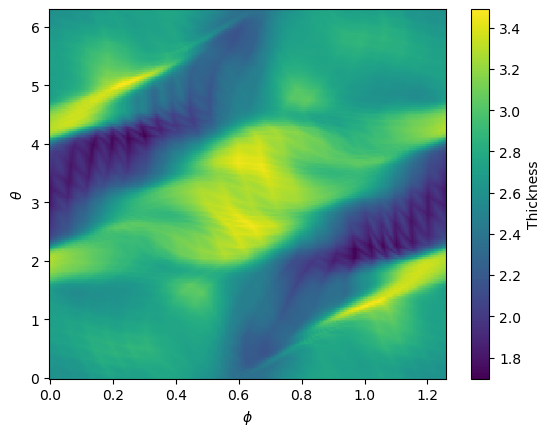
Using this thickness matrix, we can convert it to a VMEC representation, with equal arclength! This allows us to connect the mesh easily to a plasma mesh.

flux_surface_extended = jsb.flux_surfaces.create_extended_flux_surface_d_interp_equal_arclength(flux_surface_no_phi, thickness_matrix, n_theta = 50, n_phi = 60, n_theta_s_arclength=100)

extended_mesh = jsb.flux_surfaces.mesh_surfaces_closed(flux_surface_extended, 1.0, 2.0, jsb.flux_surfaces.ToroidalExtent.full_module(flux_surface_extended), 50, 60, 10)

fig = go.Figure()

add_mesh_to_plotly(fig, mesh, mesh_kwargs={"color": "lightblue", "opacity": 1.0, "name": "RMF"})
add_mesh_to_plotly(fig, extended_mesh, mesh_kwargs={"color": "lightgreen", "opacity": 1.0, "name": "Extended Flux Surface"})
add_wireframe_to_plotly(fig, extended_mesh)
fig.update_layout(height=500, width=1200)
fig.update_layout(dict(scene=dict(aspectmode='data')), width = 1200, height=700)